There are different ways to plot apparent resistivities obtained from measurements with gradient array
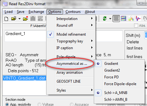
x2ipi supports three different methods for visualization of such data. One has to chose the way he wants to plot the apparent resistivity before loading the .dat file (Res2Dinv format) in "Menu - Options - Asymmetrical as ..."
|
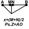
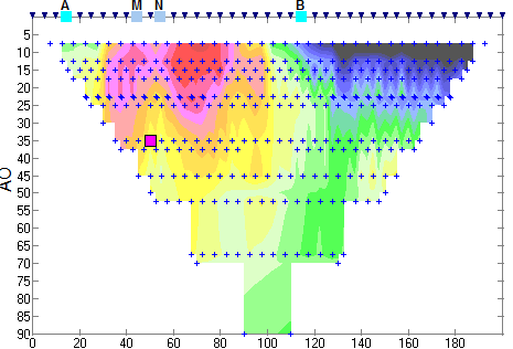
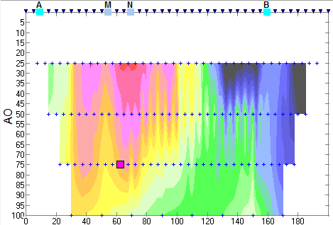
Variant 1. Gradient pseudo depth = Min(AO,OB) | |
|
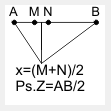
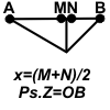
Variant 2. Gradient2 pseudo depth = AB/2 | |
|
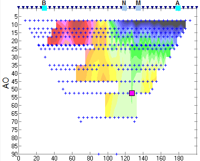
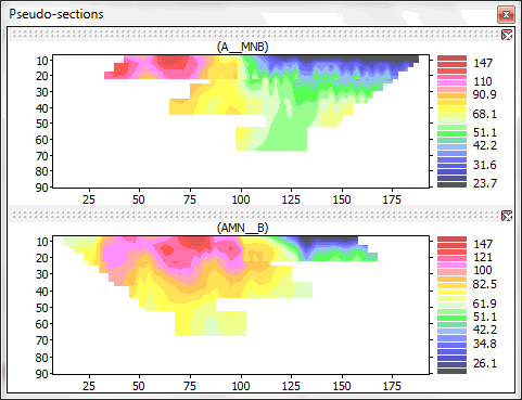
Variant 3. Force PD (Pole-Dipole analogue) Two pseudosections. |
The third way (Force PD) divides data into two pseodosections (A_MNB and AMN_B). These are plotted just like forward and reversed pole-dipole arrays.
Notice:
.dat file can contain data from different arrays. As long as Schlumberger data is in the file it will be plotted like pole-dipole. The resulting plot for Schlumberger depends on menu option: "Options - Asymmetrical as ... - Schl->A_MNB or Schl->A_MNB"
Write first comment